A Design Concept of Forecasting Software for Normalized Vector Autoregressions with Fat Tails and Stochastic Volatility
Brown Bag Seminar, University of Melbourne
Fei Shang
Guangdong University of Foreign Studies
Xiaolei (Adam) Wang
University of Melbourne
Tomasz Woźniak
University of Melbourne
Introduction
The Importance of Forecasting
- Macroeconomic forecasting is crucial for policy-makers, businesses, and researchers.
- Complex properties of macroeconomic and financial time series require scalable dynamic system modelling.
- Important decisions require robust forecasting models that adapt to unprecedented shocks and volatility (e.g., GFC, COVID-19).
Challenges
- Practical usability faces challenges from numerical complexity.
- Handling Bayesian hierarchical and non-linear modelling is numerically demanding.
- Point and density forecasting handle measurements and latent processes jointly, resulting in high dimensionality of numerical integration.
A Suite of R Packages
- We present a suite of R packages designed for forecasting using Vector Autoregressions (VARs) with Stochastic Volatility (SV) and Student-t errors.
bsvars: heteroskedastic structural VARs.bsvarSIGNs: hierarchical VARs for post-COVID forecasting.bvars: flexible VAR model.
Software Features
- Deliberate selection of modelling approaches representing commonly used specifications.
- Fast computations relying on algorithms written in C++.
- Supported by adaptation of frontier econometric and numerical methods.
- Object-oriented programming for handling multi-layered inputs and outputs.
- Coherent forecasting workflows enabling customisation and transparency.
A Suite of Predictive Models
The VAR Equation
- Our packages feature non-normal, heteroskedastic, structural, and reduced-form VARs with hierarchical priors.
- All models share the VAR equation with lag order \(p\) specified for the \(N\)-vector of dependent variables \(\mathbf{y}_t\): \[ \mathbf{y}_t = \mathbf{A}_1 \mathbf{y}_{t-1} + \ldots + \mathbf{A}_p \mathbf{y}_{t-p} + \mathbf{A}_d \mathbf{d}_{t} + \boldsymbol{\epsilon}_t \]
- Or more compactly: \(\mathbf{y}_t = \mathbf{A}\mathbf{x}_t + \boldsymbol{\epsilon}_t\).
Conditional Normality
- Predictive density’s conditional normality given past information and latent processes:
- Reduced-form: \[ \mathbf{y}_t \mid \mathbf{x}_{t}, \mathbf{A}, \boldsymbol\Sigma, \sigma_t^2, \lambda_t \sim N\left(\mathbf{A}\mathbf{x}_t, \sigma_t^2\lambda_t\boldsymbol\Sigma\right) \]
- Structural-form: \[ \mathbf{y}_t \mid \mathbf{x}_{t}, \mathbf{A}, \mathbf{B}, \boldsymbol\sigma_t^2, \boldsymbol\lambda_t \sim N\left(\mathbf{A}\mathbf{x}_t, \mathbf{B}^{-1}\text{diag}\left(\boldsymbol\sigma_t^2\right)\text{diag}\left(\boldsymbol\lambda_t\right)\mathbf{B}^{-1\prime}\right) \]
Stochastic Volatility (SV)
- Centred SV: \[ \sigma_t^2 = \exp(h_t), \quad h_t = \rho h_{t-1} + \eta_t, \quad \eta_t \sim N(0, \omega^2) \]
- Non-centred SV: \[ \sigma_t^2 = \exp(\omega h_t), \quad h_t = \rho h_{t-1} + \eta_t, \quad \eta_t \sim N(0, 1) \]
- Non-centred SV ensures normalisation around the homoskedastic case (\(\sigma_t^2 = 1\)).
Student-t Predictive Density
- Independent process \(\lambda_t\) implies Student’s t predictive density: \[ \lambda_t\mid\nu \sim IG2\left(\nu - 2, \nu\right) \]
- The prior scale restricts the prior expectation of \(\lambda_t\) to 1.
- We restrict the scale of the inverse gamma full conditional posterior to ensure that the posterior expectation \(\mathbb{E}[u_{n.t}^2] = 1\).
- Normalising VAR models results in numerically stable and scalable algorithms.
Bayesian Forecasting
- Predictive density: \[ \begin{aligned} p\left(\mathbf{y}_{T+1}\mid \mathbf{Y}_{T} \right) &= \int p\left(\mathbf{y}_{T+1}\mid \mathbf{Y}_{T}, \boldsymbol\theta, \sigma_{T+1}^2, \lambda_{T+1}\right) \\ &\quad \times p\left(\sigma_{T+1}^2\mid \mathbf{Y}_{T}, \boldsymbol\theta\right) p\left(\lambda_{T+1}\mid \mathbf{Y}_{T}, \boldsymbol\theta\right) p\left(\boldsymbol\theta \mid \mathbf{Y}_{T}\right) d\left(\boldsymbol\theta, \sigma_{T+1}^2, \lambda_{T+1}\right) \end{aligned} \]
- Computed numerically to obtain \(S\) draws from the predictive density.
- Can be used to report forecast summaries and density forecasting performance.
Forecasting Software Features
C++ Algorithms
- Combines fast algorithms in C++ with the convenience of R.
Rcppautomates compilation and linking of C++ code.- Heavy reliance on linear algebra via
RcppArmadillo. - C++ algorithms provide substantial speedups over equivalent R code (e.g., 33% faster for random number generation).
Numerical Methods
- Kronecker products and equation-by-equation sampling reduce the burden of high-dimensional matrix inversions.
- Fast row-by-row Gibbs sampler for structural matrices.
- Non-linear SV models are approximated by a 10-component conditionally Gaussian normal mixture.
- Ancillarity-sufficiency interweaving strategy speeds up MCMC convergence.
Handling Inputs and Outputs
- Object-oriented programming using
R6combines simplicity with customisation. - Separation of model specification and estimation for transparency.
- The
BSVARSVobjectspecincludes:spec$data_matricesspec$priorspec$identificationspec$starting_values
Forecasting Workflows
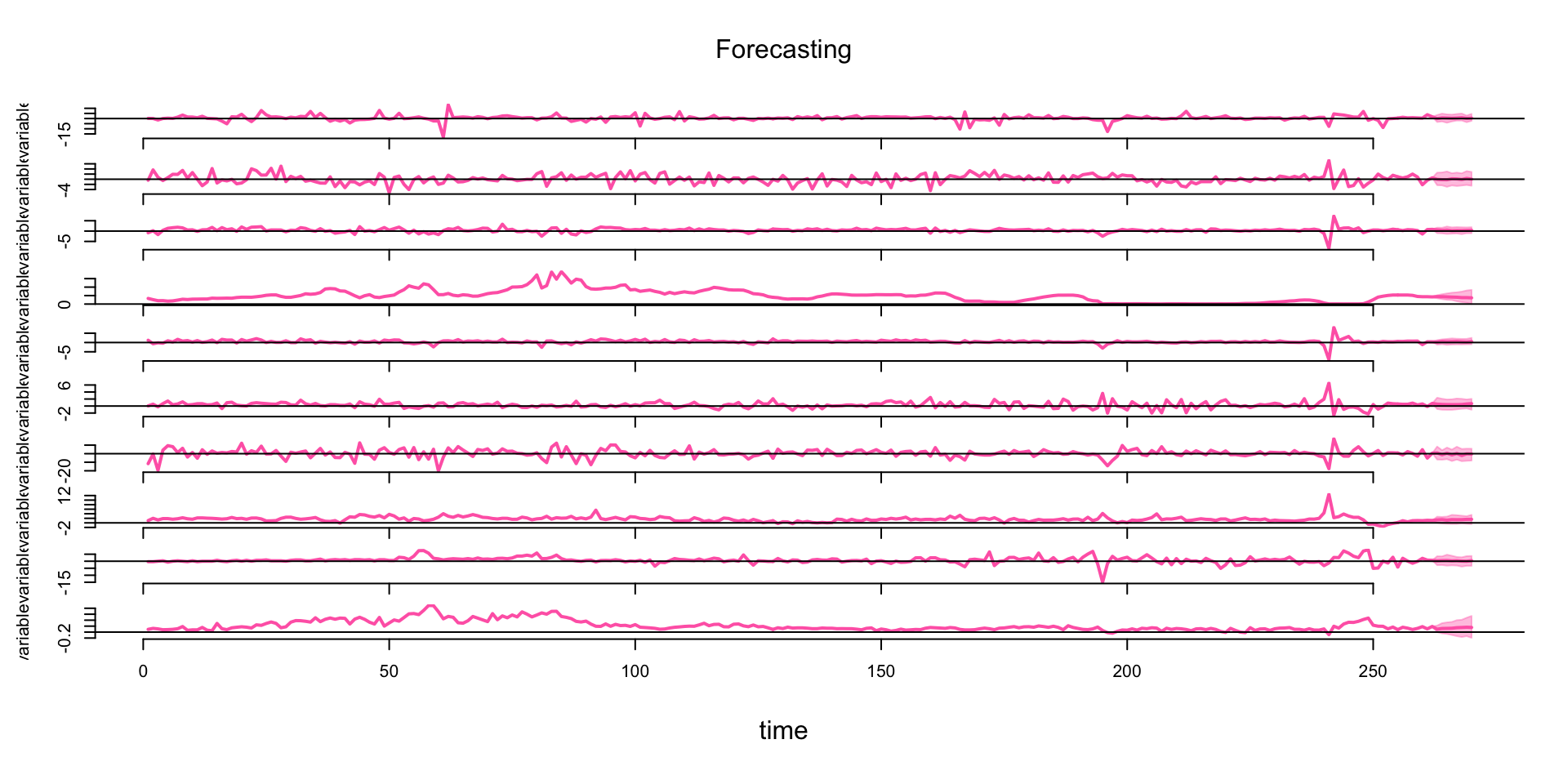
- Unified workflow around generic verbs:
estimate,forecast,compute,verify,plot,summary. - Can be implemented using the pipe operator
|>:
Post-COVID Forecasting of a Monetary-Fiscal System
Post-COVID Forecasting
- Expanding-window recursive forecasting for a 10-variable quarterly system.
- Variables: Tax revenue, government spending, GDP, federal funds rate, consumption, real wages, investment, M2, PPI, GDP deflator.
- Period: Q1 1959 to Q3 2025 (origin: Q4 2020).
- Horizons: 1-quarter (\(h=1\)) and 1-year (\(h=4\)).
- Metrics: Predictive log-score (PLS) and mean absolute scaled error (MASE).
Models in Comparison
- 19 models differing by:
- Volatility: non-centred SV, centred SV, homoskedastic (const), COVID-specific.
- Distribution: Normal (norm) or Student-t (t).
- Structure: Structural vs. Reduced-form.
- Order Invariance: Unrestricted matrix (OI) vs. lower-triangular (LT).
Forecasting Performance Table
| id | package | volatility | distr. | order | \(h=1\) PLS | \(h=1\) MASE | \(h=4\) PLS | \(h=4\) MASE |
|---|---|---|---|---|---|---|---|---|
| 1 | bsvars | ncSV | norm | OI | -13.50 | 0.97 | -18.38 | 1.37 |
| 2 | ncSV | norm | LT | -13.08 | 0.95 | -16.99 | 1.37 | |
| 3 | ncSV | t | OI | -13.61 | 0.97 | -17.91 | 1.37 | |
| 4 | ncSV | t | LT | -13.26 | 0.96 | -17.11 | 1.37 | |
| 5 | cSV | norm | OI | -13.43 | 0.96 | -17.72 | 1.39 | |
| 6 | cSV | norm | LT | -13.21 | 0.95 | -17.11 | 1.39 | |
| 7 | cSV | t | OI | -13.62 | 0.96 | -17.89 | 1.39 | |
| 8 | cSV | t | LT | -13.41 | 0.96 | -17.63 | 1.38 | |
| 9 | const | norm | LT | -15.08 | 1.05 | -18.23 | 1.45 | |
| 10 | const | t | LT | -14.11 | 0.97 | -17.21 | 1.38 | |
| 11 | const | t | OI | -14.46 | 0.99 | -18.33 | 1.39 | |
| 12 | bvars | ncSV | norm | OI | -15.11 | 1.28 | -17.80 | 1.62 |
| 13 | ncSV | t | OI | -15.22 | 1.16 | -18.05 | 1.51 | |
| 14 | cSV | norm | OI | -15.07 | 1.25 | -18.25 | 1.53 | |
| 15 | cSV | t | OI | -15.32 | 1.15 | -18.15 | 1.51 | |
| 16 | const | norm | OI | -17.13 | 1.22 | -19.40 | 1.55 | |
| 17 | const | t | OI | -15.37 | 1.16 | -18.06 | 1.51 | |
| 18 | bsvarSIGNs | COVID | norm | OI | -16.19 | 1.10 | -18.76 | 1.39 |
| 19 | const | norm | OI | -15.94 | 1.10 | -17.80 | 1.31 |
Forecasting Results Summary
- Comparison based on average exponentiated PLS and average MASE.
- Non-centred SV models outperform centred SV models.
- Raises average exponentiated PLS by ~6% at \(h=1\) and 15% at \(h=4\).
- Structural models outperform reduced-form models.
- Lower-triangular models outperform order-invariant structural models.
- Student-t distributed models outperform normal models on average.
- For point forecast accuracy (MASE), alternative SV and order-invariance specifications yield similar performance.
Conclusions
Conclusions
- Presented a suite of open-source packages designed to provide a unified framework for Bayesian VAR forecasting.
- Novel combination of features enables scalable and reproducible predictions using normalised heteroskedastic non-Gaussian models.
- Empirical results emphasise the importance of our software design to obtain precise forecasts.