Forecasting using Bayesian Structural Vector Autoregression

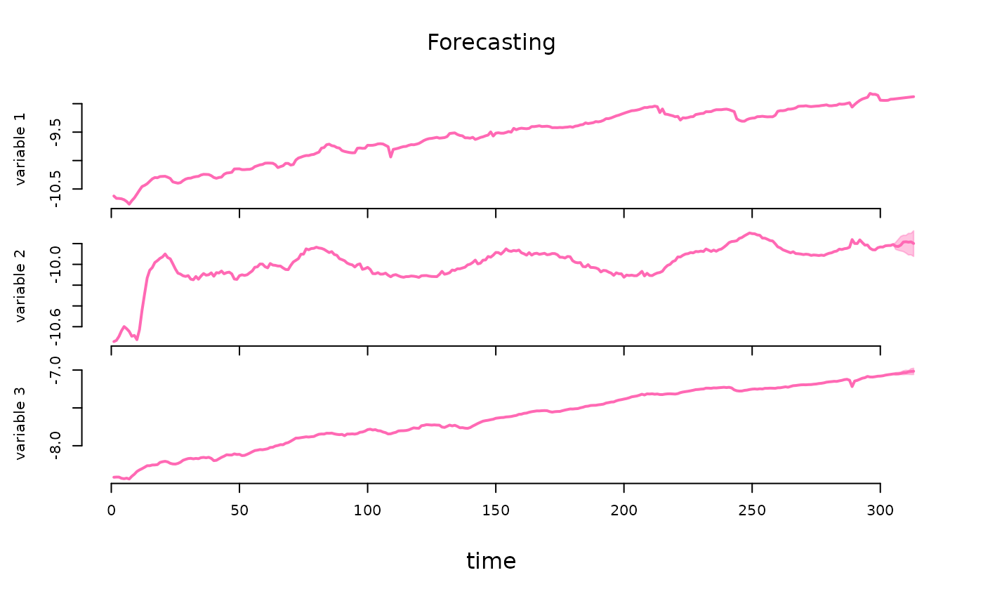
Samples from the joint predictive density of all of the dependent variables for models at forecast horizons from 1 to horizon specified as an argument of the function.

Usage

# S3 method for class 'PosteriorBSVAR'
forecast(
  object,
  horizon = 1,
  exogenous_forecast = NULL,
  conditional_forecast = NULL,
  ...
)

Arguments

object: posterior estimation outcome - an object of class PosteriorBSVAR obtained by running the estimate function.
horizon: a positive integer, specifying the forecasting horizon.
exogenous_forecast: a matrix of dimension horizon x d containing forecasted values of the exogenous variables.
conditional_forecast: a horizon x N matrix with forecasted values for selected variables. It should only contain numeric or NA values. The entries with NA values correspond to the values that are forecasted conditionally on the realisations provided as numeric values.
...: not used

Value

A list of class Forecasts containing the draws from the predictive density and for heteroskedastic models the draws from the predictive density of structural shocks conditional standard deviations and data. The output elements include:

forecasts: an NxTxS array with the draws from predictive density
Y: an \(NxT\) matrix with the data on dependent variables
forecast_mean: an NxTxS array with the mean of the predictive density
forecast_covariance: an NxTxS array with the covariance of the predictive density

Author

Tomasz Woźniak wozniak.tom@pm.me

Examples

specification  = specify_bsvar$new(us_fiscal_lsuw)
#> The identification is set to the default option of lower-triangular structural matrix.
burn_in        = estimate(specification, 5)
#> **************************************************|
#> bsvars: Bayesian Structural Vector Autoregressions|
#> **************************************************|
#>  Gibbs sampler for the SVAR model                 |
#> **************************************************|
#>  Progress of the MCMC simulation for 5 draws
#>     Every draw is saved via MCMC thinning
#>  Press Esc to interrupt the computations
#> **************************************************|
posterior      = estimate(burn_in, 5)
#> **************************************************|
#> bsvars: Bayesian Structural Vector Autoregressions|
#> **************************************************|
#>  Gibbs sampler for the SVAR model                 |
#> **************************************************|
#>  Progress of the MCMC simulation for 5 draws
#>     Every draw is saved via MCMC thinning
#>  Press Esc to interrupt the computations
#> **************************************************|
predictive     = forecast(posterior, 4)

# workflow with the pipe |>
############################################################
us_fiscal_lsuw |>
  specify_bsvar$new() |>
  estimate(S = 5) |> 
  estimate(S = 5) |> 
  forecast(horizon = 4) -> predictive
#> The identification is set to the default option of lower-triangular structural matrix.
#> **************************************************|
#> bsvars: Bayesian Structural Vector Autoregressions|
#> **************************************************|
#>  Gibbs sampler for the SVAR model                 |
#> **************************************************|
#>  Progress of the MCMC simulation for 5 draws
#>     Every draw is saved via MCMC thinning
#>  Press Esc to interrupt the computations
#> **************************************************|
#> **************************************************|
#> bsvars: Bayesian Structural Vector Autoregressions|
#> **************************************************|
#>  Gibbs sampler for the SVAR model                 |
#> **************************************************|
#>  Progress of the MCMC simulation for 5 draws
#>     Every draw is saved via MCMC thinning
#>  Press Esc to interrupt the computations
#> **************************************************|

# conditional forecasting using a model with exogenous variables
############################################################
specification  = specify_bsvar$new(us_fiscal_lsuw, exogenous = us_fiscal_ex)
#> The identification is set to the default option of lower-triangular structural matrix.
burn_in        = estimate(specification, 5)
#> **************************************************|
#> bsvars: Bayesian Structural Vector Autoregressions|
#> **************************************************|
#>  Gibbs sampler for the SVAR model                 |
#> **************************************************|
#>  Progress of the MCMC simulation for 5 draws
#>     Every draw is saved via MCMC thinning
#>  Press Esc to interrupt the computations
#> **************************************************|
posterior      = estimate(burn_in, 5)
#> **************************************************|
#> bsvars: Bayesian Structural Vector Autoregressions|
#> **************************************************|
#>  Gibbs sampler for the SVAR model                 |
#> **************************************************|
#>  Progress of the MCMC simulation for 5 draws
#>     Every draw is saved via MCMC thinning
#>  Press Esc to interrupt the computations
#> **************************************************|

# forecast 2 years ahead
predictive     = forecast(
                    posterior, 
                    horizon = 8,
                    exogenous_forecast = us_fiscal_ex_forecasts,
                    conditional_forecast = us_fiscal_cond_forecasts
                  )
summary(predictive)
#>  **************************************************|
#>  bsvars: Bayesian Structural Vector Autoregressions|
#>  **************************************************|
#>    Posterior summary of forecasts                  |
#>  **************************************************|
#> $variable1
#>        mean sd 5% quantile 95% quantile
#> 1 -8.914237  0   -8.914237    -8.914237
#> 2 -8.908921  0   -8.908921    -8.908921
#> 3 -8.903604  0   -8.903604    -8.903604
#> 4 -8.898288  0   -8.898288    -8.898288
#> 5 -8.892971  0   -8.892971    -8.892971
#> 6 -8.887655  0   -8.887655    -8.887655
#> 7 -8.882338  0   -8.882338    -8.882338
#> 8 -8.877022  0   -8.877022    -8.877022
#> 
#> $variable2
#>        mean         sd 5% quantile 95% quantile
#> 1 -9.820603 0.03086056   -9.862634    -9.798432
#> 2 -9.822402 0.04101902   -9.870001    -9.775046
#> 3 -9.843243 0.02401174   -9.872130    -9.819634
#> 4 -9.852286 0.03148237   -9.889824    -9.818935
#> 5 -9.826167 0.03807344   -9.866884    -9.779551
#> 6 -9.817373 0.05242236   -9.876198    -9.756273
#> 7 -9.812346 0.04289914   -9.847883    -9.758555
#> 8 -9.817585 0.03946899   -9.847468    -9.763915
#> 
#> $variable3
#>        mean         sd 5% quantile 95% quantile
#> 1 -7.036484 0.03803271   -7.074954    -6.988231
#> 2 -7.020970 0.05852565   -7.085975    -6.951426
#> 3 -7.005532 0.05045013   -7.060817    -6.946847
#> 4 -7.003896 0.06806594   -7.075618    -6.926386
#> 5 -7.010716 0.08237156   -7.104411    -6.925612
#> 6 -7.003595 0.09733435   -7.115237    -6.893173
#> 7 -6.995018 0.09854849   -7.105950    -6.888221
#> 8 -6.989971 0.10518358   -7.090396    -6.858711
#> 

# workflow with the pipe |>
############################################################
us_fiscal_lsuw |>
  specify_bsvar$new( exogenous = us_fiscal_ex) |>
  estimate(S = 5) |> 
  estimate(S = 5) |> 
  forecast(
    horizon = 8,
    exogenous_forecast = us_fiscal_ex_forecasts,
    conditional_forecast = us_fiscal_cond_forecasts
  ) |> plot()
#> The identification is set to the default option of lower-triangular structural matrix.
#> **************************************************|
#> bsvars: Bayesian Structural Vector Autoregressions|
#> **************************************************|
#>  Gibbs sampler for the SVAR model                 |
#> **************************************************|
#>  Progress of the MCMC simulation for 5 draws
#>     Every draw is saved via MCMC thinning
#>  Press Esc to interrupt the computations
#> **************************************************|
#> **************************************************|
#> bsvars: Bayesian Structural Vector Autoregressions|
#> **************************************************|
#>  Gibbs sampler for the SVAR model                 |
#> **************************************************|
#>  Progress of the MCMC simulation for 5 draws
#>     Every draw is saved via MCMC thinning
#>  Press Esc to interrupt the computations
#> **************************************************|