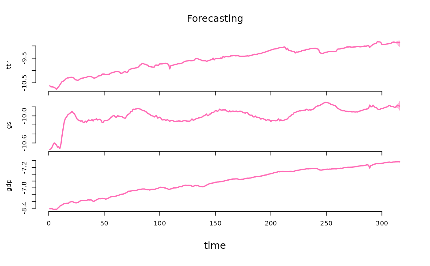
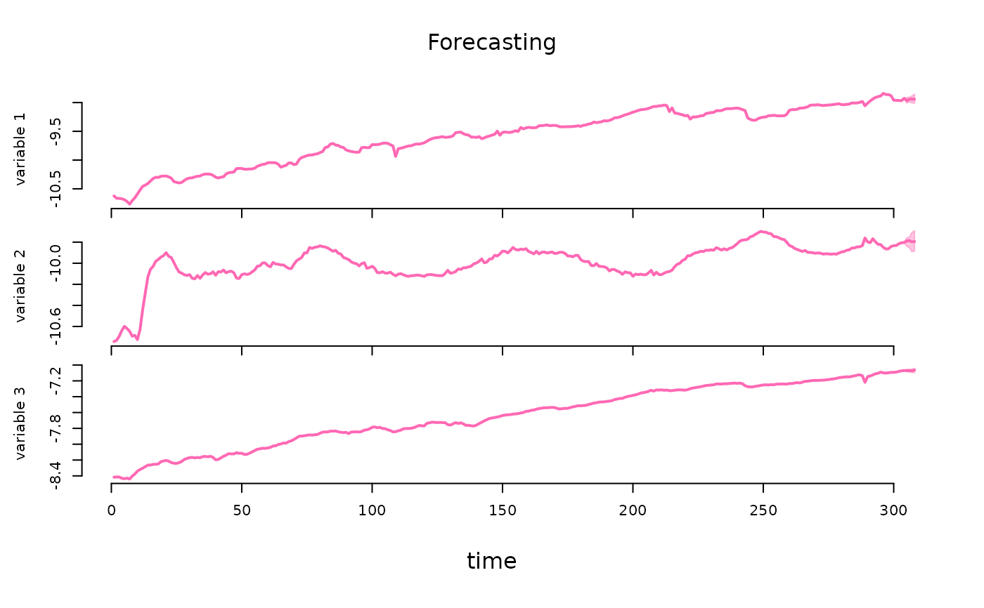
Plots of fitted values of dependent variables including their median and percentiles.
Arguments
- x
an object of class Forecasts obtained using the
forecast()function containing posterior draws of fitted values of dependent variables.- probability
a parameter determining the interval to be plotted. The interval stretches from the
0.5 * (1 - probability)to1 - 0.5 * (1 - probability)percentile of the posterior distribution.- data_in_plot
a fraction value in the range (0, 1) determining how many of the last observations in the data should be plotted with the forecasts.
- col
a colour of the plot line and the ribbon
- main
an alternative main title for the plot
- xlab
an alternative x-axis label for the plot
- mar.multi
the default
marargument setting ingraphics::par. Modify with care!- oma.multi
the default
omaargument setting ingraphics::par. Modify with care!- ...
additional arguments affecting the summary produced.
Author
Tomasz Woźniak wozniak.tom@pm.me
Examples
specification = specify_bsvar$new(us_fiscal_lsuw) # specify model
#> The identification is set to the default option of lower-triangular structural matrix.
burn_in = estimate(specification, 5) # run the burn-in
#> **************************************************|
#> bsvars: Bayesian Structural Vector Autoregressions|
#> **************************************************|
#> Gibbs sampler for the SVAR model |
#> **************************************************|
#> Progress of the MCMC simulation for 5 draws
#> Every draw is saved via MCMC thinning
#> Press Esc to interrupt the computations
#> **************************************************|
posterior = estimate(burn_in, 5) # estimate the model
#> **************************************************|
#> bsvars: Bayesian Structural Vector Autoregressions|
#> **************************************************|
#> Gibbs sampler for the SVAR model |
#> **************************************************|
#> Progress of the MCMC simulation for 5 draws
#> Every draw is saved via MCMC thinning
#> Press Esc to interrupt the computations
#> **************************************************|
# compute forecasts
fore = forecast(posterior, horizon = 4)
plot(fore) # plot forecasts
 # workflow with the pipe |>
############################################################
us_fiscal_lsuw |>
specify_bsvar$new() |>
estimate(S = 5) |>
estimate(S = 5) |>
forecast(horizon = 4) |>
plot()
#> The identification is set to the default option of lower-triangular structural matrix.
#> **************************************************|
#> bsvars: Bayesian Structural Vector Autoregressions|
#> **************************************************|
#> Gibbs sampler for the SVAR model |
#> **************************************************|
#> Progress of the MCMC simulation for 5 draws
#> Every draw is saved via MCMC thinning
#> Press Esc to interrupt the computations
#> **************************************************|
#> **************************************************|
#> bsvars: Bayesian Structural Vector Autoregressions|
#> **************************************************|
#> Gibbs sampler for the SVAR model |
#> **************************************************|
#> Progress of the MCMC simulation for 5 draws
#> Every draw is saved via MCMC thinning
#> Press Esc to interrupt the computations
#> **************************************************|
# workflow with the pipe |>
############################################################
us_fiscal_lsuw |>
specify_bsvar$new() |>
estimate(S = 5) |>
estimate(S = 5) |>
forecast(horizon = 4) |>
plot()
#> The identification is set to the default option of lower-triangular structural matrix.
#> **************************************************|
#> bsvars: Bayesian Structural Vector Autoregressions|
#> **************************************************|
#> Gibbs sampler for the SVAR model |
#> **************************************************|
#> Progress of the MCMC simulation for 5 draws
#> Every draw is saved via MCMC thinning
#> Press Esc to interrupt the computations
#> **************************************************|
#> **************************************************|
#> bsvars: Bayesian Structural Vector Autoregressions|
#> **************************************************|
#> Gibbs sampler for the SVAR model |
#> **************************************************|
#> Progress of the MCMC simulation for 5 draws
#> Every draw is saved via MCMC thinning
#> Press Esc to interrupt the computations
#> **************************************************|