Bayesian Estimation of Structural Vector Autoregressive Models

Provides fast and efficient procedures for Bayesian analysis of Structural Vector Autoregressions. This package estimates a wide range of models, including homo-, heteroskedastic and non-normal specifications. Structural models can be identified by adjustable exclusion restrictions, time-varying volatility, or non-normality, and include exclusion restrictions on autoregressive parameters. They all include a flexible three-level equation-specific local-global hierarchical prior distribution for the estimated level of shrinkage for autoregressive and structural parameters. Additionally, the package facilitates predictive and structural analyses such as impulse responses, forecast error variance and historical decompositions, forecasting, verification of heteroskedasticity and hypotheses on autoregressive parameters, and analyses of structural shocks, volatilities, and fitted values. Beautiful plots, informative summary functions, and extensive documentation including the vignette by Woźniak (2024) <doi:10.48550/arXiv.2410.15090> complement all this. The implemented techniques align closely with those presented in Lütkepohl, Shang, Uzeda, & Woźniak (2025) <doi:10.1016/j.jeconom.2025.106107>, Lütkepohl & Woźniak (2020) <doi:10.1016/j.jedc.2020.103862>, Song & Woźniak (2021) <doi:10.1093/acrefore/9780190625979.013.174>, and Woźniak & Droumaguet (2015) <doi:10.13140/RG.2.2.19492.55687>. The 'bsvars' package is aligned regarding objects, workflows, and code structure with the R package 'bsvarSIGNs' by Wang & Woźniak (2024) <doi:10.32614/CRAN.package.bsvarSIGNs>, and they constitute an integrated toolset.

Details

Models. All the SVAR models in this package are specified by two equations, including the reduced form equation: $$Y = AX + E$$ where \(Y\) is an NxT matrix of dependent variables, \(X\) is a KxT matrix of explanatory variables, \(E\) is an NxT matrix of reduced form error terms, and \(A\) is an NxK matrix of autoregressive slope coefficients and parameters on deterministic terms in \(X\).

The structural equation is given by: $$BE = U$$ where \(U\) is an NxT matrix of structural form error terms, and \(B\) is an NxN matrix of contemporaneous relationships.

Finally, all of the models share assumptions regarding the structural shocks U, namely, temporal and contemporaneous independence. They imply zero correlations and autocorrelations.

The various SVAR models estimated differ by the specification of structural shocks variances. The different models include:

• homoskedastic model with unit variances

• heteroskedastic model with non-centred Stochastic Volatility process for variances

• heteroskedastic model with centred Stochastic Volatility process for variances

• heteroskedastic model with stationary Markov switching in the variances

• heteroskedastic model with sparse Markov switching in the variances where the number of heteroskedastic components is estimated

• heteroskedastic model with stationary heterogeneous Markov switching in the variances, where each shock volatility has its own Markov process

• heteroskedastic model with sparse heterogeneous Markov switching in the variances where the number of heteroskedastic components is estimated

• heteroskedastic model with exogenous heteroskedastic regime changes in the variances

• a model with Student-t distributed structural shocks with estimated equation-specific degrees-of-freedom parameter

• non-normal model with a finite mixture of normal components and component-specific variances

• non-normal model with a sparse mixture of normal components and component-specific variances where the number of heteroskedastic components is estimated

The structural shocks can be either normally or Student-t distributed, where in the latter case the shock-specific degrees of freedom parameters are estimated.

Prior distributions. All the models feature a Minnesota prior for autoregressive parameters in matrix \(A\) and a generalised-normal distribution for the structural matrix \(B\). Both of these distributions feature a 3-level equation-specific local-global hierarchical prior that make the shrinkage estimation flexible improving the model fit and its forecasting performance.

Estimation algorithm. The models are estimated using frontier numerical methods making the Gibbs sampler fast and efficient. The estimation follows closely Lütkepohl, Shang, Uzeda, & Woźniak (2025). The sampler of the structural matrix follows Waggoner & Zha (2003), whereas that for autoregressive parameters follows Chan, Koop, Yu (2022). The specification of Markov switching heteroskedasticity is inspired by Song & Woźniak (2021), and that of Stochastic Volatility model by Kastner & Frühwirth-Schnatter (2014). The identification problems are considered in Lütkepohl, Shang, Uzeda, & Woźniak (2025) and Lütkepohl & Woźniak (2020).

Identification verification. The structural shocks can be identified through heteroskedasticity or non-normality following Lütkepohl, Shang, Uzeda, & Woźniak (2025) and Lütkepohl & Woźniak (2020). The package provides functions to verify both, homoskedasticity and normality of the structural shocks, which facilitates making probabilistic statements regarding the identification. Additionally, the package makes it possible to verify linear restrictions on autoregressive parameters.

Note

This package is currently in active development. Your comments, suggestions and requests are warmly welcome!

References

Chan, J.C.C., Koop, G, and Yu, X. (2024) Large Order-Invariant Bayesian VARs with Stochastic Volatility. Journal of Business & Economic Statistics, 42, doi:10.1080/07350015.2023.2252039 .

Kastner, G. and Frühwirth-Schnatter, S. (2014) Ancillarity-Sufficiency Interweaving Strategy (ASIS) for Boosting MCMC Estimation of Stochastic Volatility Models. Computational Statistics & Data Analysis, 76, 408–423, doi:10.1016/j.csda.2013.01.002 .

Lütkepohl, H., Shang, F., Uzeda, L., and Woźniak, T. (2025) Partial identification of structural vector autoregressions with non-centred stochastic volatility. Journal of Econometrics, 1–18, doi:10.1016/j.jeconom.2025.106107 .

Lütkepohl, H., and Woźniak, T., (2020) Bayesian Inference for Structural Vector Autoregressions Identified by Markov-Switching Heteroskedasticity. Journal of Economic Dynamics and Control 113, 103862, doi:10.1016/j.jedc.2020.103862 .

Song, Y., and Woźniak, T. (2021) Markov Switching Heteroskedasticity in Time Series Analysis. In: Oxford Research Encyclopedia of Economics and Finance. Oxford University Press, doi:10.1093/acrefore/9780190625979.013.174 .

Waggoner, D.F., and Zha, T., (2003) A Gibbs sampler for structural vector autoregressions. Journal of Economic Dynamics and Control, 28, 349–366, doi:10.1016/S0165-1889(02)00168-9 .

See also

Useful links:

• https://bsvars.org/bsvars/

• Report bugs at https://github.com/bsvars/bsvars/issues

Author

Tomasz Woźniak wozniak.tom@pm.me

Examples

spec  = specify_bsvar_sv$new(         # specify the model
          us_fiscal_lsuw, 
          exogenous = us_fiscal_ex
        )
#> The identification is set to the default option of lower-triangular structural matrix.
burn  = estimate(spec, 5)             # run the burn-in
#> **************************************************|
#> bsvars: Bayesian Structural Vector Autoregressions|
#> **************************************************|
#>  Gibbs sampler for the SVAR-SV model              |
#>    Non-centred SV model is estimated              |
#> **************************************************|
#>  Progress of the MCMC simulation for 5 draws
#>     Every draw is saved via MCMC thinning
#>  Press Esc to interrupt the computations
#> **************************************************|
post  = estimate(burn, 10)            # estimate the model
#> **************************************************|
#> bsvars: Bayesian Structural Vector Autoregressions|
#> **************************************************|
#>  Gibbs sampler for the SVAR-SV model              |
#>    Non-centred SV model is estimated              |
#> **************************************************|
#>  Progress of the MCMC simulation for 10 draws
#>     Every draw is saved via MCMC thinning
#>  Press Esc to interrupt the computations
#> **************************************************|
irf   = compute_impulse_responses(    # compute impulse responses
          post, 
          horizon = 2
         )

# compute forecast error variance decomposition one year ahead
fevd  = compute_variance_decompositions(post, horizon = 4)

# workflow with the pipe |>
############################################################
us_fiscal_lsuw |>
  specify_bsvar_sv$new(exogenous = us_fiscal_ex) |>
  estimate(S = 5) |> 
  estimate(S = 10) |> 
  compute_variance_decompositions(horizon = 4) -> fevds
#> The identification is set to the default option of lower-triangular structural matrix.
#> **************************************************|
#> bsvars: Bayesian Structural Vector Autoregressions|
#> **************************************************|
#>  Gibbs sampler for the SVAR-SV model              |
#>    Non-centred SV model is estimated              |
#> **************************************************|
#>  Progress of the MCMC simulation for 5 draws
#>     Every draw is saved via MCMC thinning
#>  Press Esc to interrupt the computations
#> **************************************************|
#> **************************************************|
#> bsvars: Bayesian Structural Vector Autoregressions|
#> **************************************************|
#>  Gibbs sampler for the SVAR-SV model              |
#>    Non-centred SV model is estimated              |
#> **************************************************|
#>  Progress of the MCMC simulation for 10 draws
#>     Every draw is saved via MCMC thinning
#>  Press Esc to interrupt the computations
#> **************************************************|

# conditional forecasting using a model with exogenous variables
############################################################
us_fiscal_lsuw |>
  specify_bsvar_sv$new(exogenous = us_fiscal_ex) |>
  estimate(S = 5) |> 
  estimate(S = 10) -> post
#> The identification is set to the default option of lower-triangular structural matrix.
#> **************************************************|
#> bsvars: Bayesian Structural Vector Autoregressions|
#> **************************************************|
#>  Gibbs sampler for the SVAR-SV model              |
#>    Non-centred SV model is estimated              |
#> **************************************************|
#>  Progress of the MCMC simulation for 5 draws
#>     Every draw is saved via MCMC thinning
#>  Press Esc to interrupt the computations
#> **************************************************|
#> **************************************************|
#> bsvars: Bayesian Structural Vector Autoregressions|
#> **************************************************|
#>  Gibbs sampler for the SVAR-SV model              |
#>    Non-centred SV model is estimated              |
#> **************************************************|
#>  Progress of the MCMC simulation for 10 draws
#>     Every draw is saved via MCMC thinning
#>  Press Esc to interrupt the computations
#> **************************************************|
  
 post |> forecast(
    horizon = 8,
    exogenous_forecast = us_fiscal_ex_forecasts,
    conditional_forecast = us_fiscal_cond_forecasts
  ) -> pred
  
  pred |> summary()
#>  **************************************************|
#>  bsvars: Bayesian Structural Vector Autoregressions|
#>  **************************************************|
#>    Posterior summary of forecasts                  |
#>  **************************************************|
#> $variable1
#>        mean sd 5% quantile 95% quantile
#> 1 -8.860009  0   -8.860009    -8.860009
#> 2 -8.854638  0   -8.854638    -8.854638
#> 3 -8.849268  0   -8.849268    -8.849268
#> 4 -8.843897  0   -8.843897    -8.843897
#> 5 -8.838526  0   -8.838526    -8.838526
#> 6 -8.833155  0   -8.833155    -8.833155
#> 7 -8.827784  0   -8.827784    -8.827784
#> 8 -8.822413  0   -8.822413    -8.822413
#> 
#> $variable2
#>        mean         sd 5% quantile 95% quantile
#> 1 -9.821451 0.02022207   -9.851002    -9.799105
#> 2 -9.813261 0.04392924   -9.882530    -9.766174
#> 3 -9.815333 0.04840641   -9.883271    -9.753411
#> 4 -9.812353 0.04379210   -9.867559    -9.761569
#> 5 -9.812701 0.04975541   -9.878213    -9.753131
#> 6 -9.801666 0.04277242   -9.849487    -9.738063
#> 7 -9.790058 0.05588213   -9.868347    -9.732756
#> 8 -9.793242 0.05227908   -9.868112    -9.737538
#> 
#> $variable3
#>        mean         sd 5% quantile 95% quantile
#> 1 -7.057478 0.01309865   -7.077604    -7.041517
#> 2 -7.043414 0.01636002   -7.064431    -7.024429
#> 3 -7.029661 0.02940310   -7.066260    -6.991101
#> 4 -7.035069 0.02834075   -7.074827    -7.003542
#> 5 -7.027991 0.03158928   -7.070093    -6.989848
#> 6 -7.016603 0.04205727   -7.067684    -6.959491
#> 7 -7.010115 0.03698460   -7.046770    -6.952263
#> 8 -7.005864 0.04576517   -7.050678    -6.930307
#> 
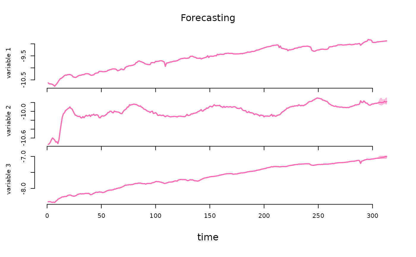
  pred |> plot(probability = 0.68)

  
# estimation of a model with exogeneity restrictions on the  autoregressive matrix
#############################################################
A = matrix(TRUE, 3, 7)
A[1,3] = A[1,6] = FALSE
us_fiscal_lsuw |>
  specify_bsvar_sv$new(p = 2, A = A) |>
  estimate(S = 5) |> 
  estimate(S = 10) -> post
#> The identification is set to the default option of lower-triangular structural matrix.
#> **************************************************|
#> bsvars: Bayesian Structural Vector Autoregressions|
#> **************************************************|
#>  Gibbs sampler for the SVAR-SV model              |
#>    Non-centred SV model is estimated              |
#> **************************************************|
#>  Progress of the MCMC simulation for 5 draws
#>     Every draw is saved via MCMC thinning
#>  Press Esc to interrupt the computations
#> **************************************************|
#> **************************************************|
#> bsvars: Bayesian Structural Vector Autoregressions|
#> **************************************************|
#>  Gibbs sampler for the SVAR-SV model              |
#>    Non-centred SV model is estimated              |
#> **************************************************|
#>  Progress of the MCMC simulation for 10 draws
#>     Every draw is saved via MCMC thinning
#>  Press Esc to interrupt the computations
#> **************************************************|
post |> summary()
#>  **************************************************|
#>  bsvars: Bayesian Structural Vector Autoregressions|
#>  **************************************************|
#>    Posterior summary of the parameters             |
#>  **************************************************|
#> $B
#> $B$equation1
#>             mean          sd 5% quantile 95% quantile
#> B[1,1] 0.1609526 0.009724098   0.1482506    0.1745887
#> 
#> $B$equation2
#>             mean        sd 5% quantile 95% quantile
#> B[2,1] -17.17922 0.4086497   -17.73462    -16.70508
#> B[2,2]  39.79082 0.9360247    38.70717     41.06400
#> 
#> $B$equation3
#>             mean       sd 5% quantile 95% quantile
#> B[3,1] -36.20602 1.318191   -38.28135    -35.16755
#> B[3,2] -15.93772 1.439007   -17.28044    -13.67225
#> B[3,3]  75.42772 2.419736    73.13755     79.13180
#> 
#> 
#> $A
#> $A$equation1
#>                  mean         sd  5% quantile 95% quantile
#> lag1_var1  0.42171673 0.10920143  0.315804147   0.59608546
#> lag1_var1 -0.06686843 0.06526409 -0.170518124   0.01027643
#> lag1_var2  0.00000000 0.00000000  0.000000000   0.00000000
#> lag2_var2 -0.09110386 0.11398995 -0.274469571   0.01811103
#> lag2_var3  0.08009973 0.05986719  0.009747408   0.17070994
#> lag2_var3  0.00000000 0.00000000  0.000000000   0.00000000
#> const      0.08925250 0.16461690 -0.159865358   0.28531654
#> 
#> $A$equation2
#>                 mean         sd 5% quantile 95% quantile
#> lag1_var1 -0.1525664 0.07764336 -0.25345208  -0.06161647
#> lag1_var1  1.3129551 0.06240304  1.23403815   1.40891955
#> lag1_var2 -0.2698253 0.18699972 -0.52549594  -0.02402277
#> lag2_var2 -0.1377315 0.07143121 -0.21915973  -0.04953971
#> lag2_var3 -0.3470453 0.05709620 -0.43706398  -0.27741432
#> lag2_var3  0.2792166 0.18925012  0.01471495   0.54165277
#> const     -0.2999137 0.12874091 -0.45550708  -0.12483533
#> 
#> $A$equation3
#>                  mean         sd 5% quantile 95% quantile
#> lag1_var1 -0.31105726 0.03705400 -0.36352538 -0.260308985
#> lag1_var1 -0.05998329 0.03796136 -0.12019431 -0.016862718
#> lag1_var2  0.73522816 0.12350453  0.57702445  0.894012777
#> lag2_var2 -0.05450381 0.03353649 -0.09983163 -0.007488511
#> lag2_var3  0.06498192 0.03386746  0.02937896  0.119054952
#> lag2_var3  0.24261808 0.11531892  0.09805008  0.388313528
#> const      0.01959770 0.09471736 -0.08775735  0.147580729
#> 
#> 
#> $hyper
#> $hyper$B
#>                            mean        sd 5% quantile 95% quantile
#> B[1,]_shrinkage        150.8314  160.4015    30.56898     446.5439
#> B[2,]_shrinkage        433.6038  275.5641   167.64254     860.3865
#> B[3,]_shrinkage        944.4309  317.4391   511.16866    1381.7308
#> B[1,]_shrinkage_scale 1319.7482  992.8173   296.42553    2795.8059
#> B[2,]_shrinkage_scale 1730.5786  911.8293   284.65481    2633.4958
#> B[3,]_shrinkage_scale 1979.1464 1343.5224   472.89148    4076.4553
#> B_global_scale         150.0590  105.8305    26.02227     308.5600
#> 
#> $hyper$A
#>                            mean        sd 5% quantile 95% quantile
#> A[1,]_shrinkage       0.2689406 0.1346945   0.1472030    0.4902040
#> A[2,]_shrinkage       0.6388779 0.3660288   0.3072325    1.2830128
#> A[3,]_shrinkage       0.3034034 0.1366203   0.1708326    0.5274419
#> A[1,]_shrinkage_scale 4.0086525 0.8401828   2.9333186    5.3358045
#> A[2,]_shrinkage_scale 6.3038629 3.3969510   3.1634492   12.1402048
#> A[3,]_shrinkage_scale 4.7680245 2.3494172   2.9847799    9.0201715
#> A_global_scale        0.6285960 0.2424468   0.4190000    1.0294173
#> 
#>