Plots historical decompositions

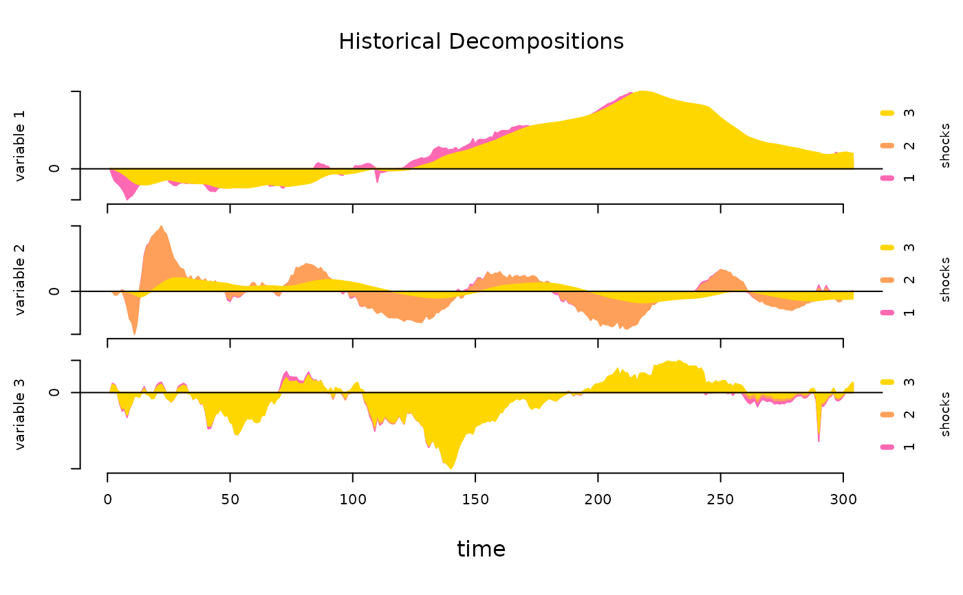
Plots of the posterior means of the historical decompositions.

Usage

# S3 method for class 'PosteriorHD'
plot(
  x,
  shock_names,
  cols,
  main,
  xlab,
  mar.multi = c(1, 4.6, 0, 4.6),
  oma.multi = c(6, 0, 5, 0),
  ...
)

Arguments

x

an object of class PosteriorHD obtained using the compute_historical_decompositions() function containing posterior draws of historical decompositions.

shock_names

a vector of length N containing names of the structural shocks.

cols

an N-vector with colours of the plot

main

an alternative main title for the plot

xlab

an alternative x-axis label for the plot

mar.multi

the default mar argument setting in graphics::par. Modify with care!

oma.multi

the default oma argument setting in graphics::par. Modify with care!

...

additional arguments affecting the summary produced.

See also

compute_historical_decompositions

Author

Tomasz Woźniak wozniak.tom@pm.me

Examples

data(us_fiscal_lsuw)                                  # upload data
set.seed(123)                                         # set seed
specification  = specify_bsvar$new(us_fiscal_lsuw)    # specify model
#> The identification is set to the default option of lower-triangular structural matrix.
burn_in        = estimate(specification, 10)          # run the burn-in
#> **************************************************|
#> bsvars: Bayesian Structural Vector Autoregressions|
#> **************************************************|
#>  Gibbs sampler for the SVAR model                 |
#> **************************************************|
#>  Progress of the MCMC simulation for 10 draws
#>     Every draw is saved via MCMC thinning
#>  Press Esc to interrupt the computations
#> **************************************************|
posterior      = estimate(burn_in, 20, thin = 1)      # estimate the model
#> **************************************************|
#> bsvars: Bayesian Structural Vector Autoregressions|
#> **************************************************|
#>  Gibbs sampler for the SVAR model                 |
#> **************************************************|
#>  Progress of the MCMC simulation for 20 draws
#>     Every draw is saved via MCMC thinning
#>  Press Esc to interrupt the computations
#> **************************************************|

# compute historical decompositions
fevd           = compute_historical_decompositions(posterior)
#> **************************************************|
#> bsvars: Bayesian Structural Vector Autoregressions|
#> **************************************************|
#>  Computing historical decomposition               |
#> **************************************************|
#>  This might take a little while :)                
#> **************************************************|
plot(fevd)                                            


# workflow with the pipe |>
############################################################
set.seed(123)
us_fiscal_lsuw |>
  specify_bsvar$new() |>
  estimate(S = 10) |> 
  estimate(S = 20, thin = 1) |> 
  compute_historical_decompositions() |>
  plot()
#> The identification is set to the default option of lower-triangular structural matrix.
#> **************************************************|
#> bsvars: Bayesian Structural Vector Autoregressions|
#> **************************************************|
#>  Gibbs sampler for the SVAR model                 |
#> **************************************************|
#>  Progress of the MCMC simulation for 10 draws
#>     Every draw is saved via MCMC thinning
#>  Press Esc to interrupt the computations
#> **************************************************|
#> **************************************************|
#> bsvars: Bayesian Structural Vector Autoregressions|
#> **************************************************|
#>  Gibbs sampler for the SVAR model                 |
#> **************************************************|
#>  Progress of the MCMC simulation for 20 draws
#>     Every draw is saved via MCMC thinning
#>  Press Esc to interrupt the computations
#> **************************************************|
#> **************************************************|
#> bsvars: Bayesian Structural Vector Autoregressions|
#> **************************************************|
#>  Computing historical decomposition               |
#> **************************************************|
#>  This might take a little while :)                
#> **************************************************|